Metagenomics
08 Jun 2023Assignment 13: Metagenomics
Background
Metagenomics is a rapidly expanding field with the power to explain microbial communities with a very high resolution by leveraging next generation sequencing data. There are applications in the clinic, ecological environments, food safety, and others. By definition, metagenomics is the study of a collection of genetic material (genomes) from a mixed community of organisms typically microbial.
Today we will walk through a common metagenomics workflow using QIIME2 (pronounced “chime”) and phyloseq by completing the following:
- Determine the various microbial communities in our samples
- Calculate the diversity within our sample (alpha diversity)
- Calculate the diversity between different sample types (beta diversity)
Acknowledgement must be paid to Professor Scott Dawson for sharing his original metagenomics lab that we have adapted for this class, to the Sundaresan Lab for sharing the data from their publication, and to former TA Kristen Beck who wrote an earlier version of the lab.
Clone your repository
Clone your Assignment_13 repository
- cd into the repository
- There will be an assignment template for today’s lab.
BIS180L 2023 shortcuts
the normal workflow would be to use Qiime to
- Cluster the 16S sequences into OTUs
- Match the OTUs against an existing database to assign taxonomy
- Export the results to a file that R can handle
- Analyze the results
In 2023 we have pre-run 1, 2, and 3 for you. The code required to install Qiime and run these steps is available at the end of this lab as a reference in case you need it later.
Download Data
Switch to your Assignment_13/input directory
Download and unzip the data files:
wget https://bis180ldata.s3.amazonaws.com/downloads/Metagenomics/MetaGenomeData.tar.gz

tar -xvzf MetaGenomeData.tar.gz
Background for our Data
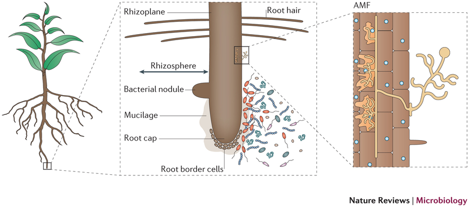
Today, we will be working with the samples collected from the rhizosphere of rice plants. The rhizosphere is an area of soil near the plant roots that contains both bacteria and other microbes associated with roots as well as secretions from the roots themselves. See diagram below from Phillppot et al., Nature, 2013.
In order to classify microbial diversity, metagenomics often relies on sequencing 16S ribosomal RNA which is the small subunit (SSU) of the prokaryotic ribosome. This region has a slow rate of evolution and therefore can be advantageous in constructing phylogenies. For this lab, samples for various soil depths and cultivars were sequenced with Illumina sequencing. The de-multiplexed reads that we will be working with are in RiceSeqs.fna, and the sample information is in RiceMappingFile.txt.
The naming conventions of the Sample IDs are a little abstract, so I have created a quick reference table for you here.
| Cultivar | Source |
|---|---|
| NE = Nipponbare Early | M = 1mm soil |
| NL = Nipponbare Late | B = root surface |
| I = IR50 | E = root inside |
| M = M104 |
* Technical replicates are indicated with 1 or 2
Explore and Quality Control Data
Often times, as bioinformaticians, we will receive data sets with little background. Sometimes the first step is to explore the raw data that we will be working with. This can help us spot inconsistencies or logical fallacies down the line when working with more automated pipelines.
In the Terminal open RiceMappingFile.txt with less to view more information about the data you are working with. This file contains information about each sample including the cultivar, treatment, and number of technical replicates. It also includes the barcodes used to identify each sample during multiplexing. Let’s use the barcodes to determine if we have an similar number of reads per sample ID.
In the RiceSeqs.fna file, barcodes for each sequence are indicated in the header with new_bc=. These barcodes are also mapped to the sample information in RiceMapping.txt. Try to determine the number of sequences present for each barcode. This can be accomplished using just Linux/Unix commands. I’ll start by giving you the tools, so you can try to piece together the command on your own.
Helpful Commands (in no particular order): cut, grep, sort, uniq and good ‘ol | to chain the commands together.
If you get stuck, highlight the hidden text underneath this sentence for one potential solution to identifying the barcodes themselves.
grep ">" RiceSeqs.fna | cut -d " " -f 4 | sort | uniq -cExercise 1:
Using information in the RiceMappingFile.txt and RiceSeqs.fna answer the following questions.
a. Are the number of sequences for each sample approximately the same or are there any outliers? If so, which samples do they belong to?
b. Could a different number of sequences per sample affect future analysis? Explain your reasoning.
Now that we’ve poked around in our raw data, let’s carry on with analyzing the microbes present in our samples.
Download Qiime Export
This is the output we would get from running Qiime to cluster and classify our OTUs. See the bottoms of the lab for the commands that generated this.
wget http://bis180ldata.s3.amazonaws.com/downloads/Metagenomics/qiime_export.tar.gz
tar -xvzf qiime_export.tar.gz
Exercise 2:
Examine the input/qiime_export/otu_class.txt file, which is a summary of the OTUs. Look at how many OTUs are found in each sample (“counts/sample detail”). Do technical replicates agree with one another? At this stage, what conclusions can you draw about the number of OTUs in these samples?
Import OTU table into R
We will use the R package phyloseq To analyze the OTU data.
First, install it (only needs to be done once).
In R:
if (!requireNamespace("BiocManager", quietly = TRUE))
    install.packages("BiocManager")

BiocManager::install("phyloseq")
You will see many warning messages go by. It is okay to ignore them.
When asked “Update all/some/none? [a/s/n]:” you can choose “n”
Load the libraries
library(phyloseq)
library(tidyverse)
Import the otu count data
otu <- read.delim("../input/qiime_export/otu_table.txt", skip=1, row.names = 1, as.is = TRUE) %>% as.matrix()
head(otu)
Import the taxonomy key
tax <- read.delim("../input/qiime_export/taxonomy.tsv", as.is = TRUE) %>%
  select(-Consensus) %>%
  mutate(Taxon = str_remove_all(Taxon, ".__| ")) %>%
  separate(Taxon, into = c("domain", "phylum", "class", "order", "family", "genus", "species"), sep = ";", fill="right")
rownames(tax) <- tax$Feature.ID
tax <- tax %>% select(-Feature.ID) %>% as.matrix()
tax[tax==""] <- NA
head(tax)
Create a data frame of sample info
sampleinfo <- data.frame(sample=colnames(otu)) %>%
  mutate(cultivar=str_sub(sample,1,1),
         cultivar={str_replace(cultivar, "M", "M104") %>%
             str_replace( "I", "IR50") %>%
             str_replace( "N", "Nipponbare")},
         time={str_extract(sample,"N(E|L)") %>%
             str_remove("N")},
         location={str_extract(sample,".[12]") %>% str_sub(1,1)},
         location={str_replace(location, "B", "rhizoplane") %>%
             str_replace("M", "rhizosphere") %>%
             str_replace("E", "endosphere")})
rownames(sampleinfo) <- sampleinfo$sample
sampleinfo <- sampleinfo %>% select(-sample)
head(sampleinfo)
Bring the OTUs and the taxonomy table together into one phyloseq object
rice.ps <- phyloseq(otu_table(otu,taxa_are_rows=TRUE), tax_table(tax), sample_data(sampleinfo))
rice.ps
Do some filtering to remove rare sequences
rice.ps.small <- filter_taxa(rice.ps, function(x) sum(x > 5) > 2, prune=TRUE) #require greater than five observation in more than two samples
rice.ps.small <- prune_taxa(complete.cases(tax_table(rice.ps.small)[,"phylum"]),  rice.ps.small) #remove taxa from unknown phylum
rice.ps.small
Use the rice.ps.small data set for the remainder of this lab unless other data set is stated
Heatmap
As we learned last week, we can rely on the human eye to help pick out patterns based on color. We are going to make a heat map of the OTUs per sample. The OTU table is visualized as a heat map where each row corresponds to an OTU and each column corresponds to a sample. The higher the relative abundance of an OTU in a sample, the more intense the color at the corresponding position in the heat map. OTUs are clustered by Bray-Curtis dissimilarity. For a refresher on biological classification, view this helpful wiki page.
plot_heatmap(rice.ps.small)
Exercise 3: Although, the resolution of the y-axis makes it impossible to read each OTU, it is still a valuable preliminary visualization. What types of information can you gain from this heat map? Are there any trends present at this stage with respect to the various samples?
Barplots
Now we’d like to visualize our data with a little higher resolution and summarize the communities by their taxonomic composition.
Use the following command to generate a boxplot to describe our samples. Here we are coloring by phylum, but we could use any level of taxonomic information
plot_bar(rice.ps.small, fill="phylum")
a line separates every OTU, which leads to a lot of black. We can get rid of the black lines with
pl <- plot_bar(rice.ps.small, fill="phylum")
pl + geom_col(aes(fill=phylum, color=phylum)) +
  scale_fill_brewer(type="qual", palette="Paired") + # better colors
  scale_color_brewer(type="qual", palette="Paired") # better colors
This is a helpful visualization but what if you want to group the bar plots by cultivar or sample location? Open the help page for plot_bar and work out how to do that. (You may also want to look at the phyloseq plot_bar tutorial)
If you prefer to look at the counts, you can use the psmelt() function to create a data frame, and then use tidyverse functions, for example:
rice.ps.small %>%
  psmelt() %>%
  group_by(phylum) %>%
  summarize(Abundance=sum(Abundance)) %>%
  arrange(desc(Abundance))
## # A tibble: 11 x 2
##    phylum            Abundance
##    <chr>                 <dbl>
##  1 Proteobacteria         8326
##  2 Myxococcota            1684
##  3 Actinobacteriota       1494
##  4 Desulfobacterota        406
##  5 Bacteroidota            350
##  6 Gemmatimonadota         334
##  7 Firmicutes              209
##  8 Fibrobacterota          197
##  9 Nitrospirota            110
## 10 Verrucomicrobiota        62
## 11 Acidobacteriota          47
Exercise 4:
a. Make a bar plot with samples grouped by location.
b. Make a table showing the phylum abundance by location (build on code above). I’ve shown what the first two rows should look like; yours should have 11 rows.
## `summarise()` has grouped output by 'location'. You can override using the `.groups` argument.
## # A tibble: 2 x 4
##   phylum           endosphere rhizoplane rhizosphere
##   <chr>                 <dbl>      <dbl>       <dbl>
## 1 Acidobacteriota           2          1          44
## 2 Actinobacteriota        857         94         543
c. When comparing by location, which single phylum is most abundant across all locations? Are there any predominant phyla greatly enriched (greater than 10-fold) in one location compared to the others?
d. Repeat a, b, and c but this time grouping by cultivar. When comparing by cultivar, is the predominant phyla consistent with that observed in Part B? Are there any predominant phyla unique to a specific cultivar? What does this indicate to you about the effect of the genotype and/or the effect of the sample location?
Now that we know a little more information about the OTUs in our sample, we’d like to calculate the diversity within a sample –the alpha diversity– and between our samples –the beta diversity.
Determine the Diversity Within a Sample
Alpha diversity tells us about the richness of species diversity within our sample. It quantifies how many taxa are in one sample and allow us to answer questions like “Are polluted environments less diverse than pristine environments?”.
There are more than two dozen different established metrics to calculate the alpha diversity. We will start with a small subset of methods. Feel free to read more details about other metrics here.
Generate plots using rice.ps for Exercises 5 and 6
plot_richness(rice.ps, measures=c("Observed", "Chao1", "Shannon"))
Exercise 5:
Is there an alpha diversity metric that estimates the sample diversity differently than the other metrics? If so, which one is it? (This is not a question about the scale of the y-axis, but the patterns of which samples show relatively high and low diversity).
Exercise 6:
Look at the help file for plot_richness and plot the samples grouped first by cultivar and then make a separate plot with them grouped by location. Do either of these categories seem to affect species diversity? Thinking back to the difference in read counts per sample, could the differences in diversity just be due to differences in sequencing depth?
Visualize the Diversity Between Samples
The definition of beta diversity has become quite contentious among ecologists. For the purpose of this lab, we will define beta diversity as the differentiation among samples which is also the practical definition QIIME uses. To quantify beta diversity, we will calculate the pairwise Bray-Curtis dissimilarity, resulting in a distance matrix. For more information about other definitions/uses of beta diversity, see the wikipedia page.
First compute the distances and compute MDS coordinates
rice.ord.small <- ordinate(rice.ps.small, method="NMDS", distance="bray")
Now plot:
pl <- plot_ordination(rice.ps, rice.ord.small, type="samples", color="cultivar", shape="location")
pl + geom_point(size=4)
Exercise 7:
a. Does cultivar or location appear to have more of an influence on the clustering?
b. Which two locations are more similar to one another? Does that make biological sense?
Exercise 8:
Four Nipponbarre samples form a distinct group separated from all other samples. Replot the data (changing the plot aesthetics) to provide an explanation.
Congratulations!
You now have learned how to do some classic metagenomics analyses.
Extras. Not needed 2023.
Install QIIME2
Quantitative Insights Into Microbial Ecology or QIIME2 is an open-source bioinformatics pipeline for performing microbiome analysis from raw DNA sequencing data. It has been cited by over 2,500 peer-reviewed journals since its publication in 2010.
In terminal:
cd ~/Downloads
wget https://repo.anaconda.com/miniconda/Miniconda3-latest-Linux-x86_64.sh
bash Miniconda3-latest-Linux-x86_64.sh #run installer for conda
eval "$(/home/exouser/miniconda3/bin/conda shell.bash hook)"
When asked, answer “yes” to agree to the license, “yes” to keep the default installation directory, and “yes” to initialize Miniconda3.
Now, close your terminal and then open a new window so that conda is active.
Next, update conda.
conda update conda
# hit enter or "y" then enter to install updates
Then, install qiime2. This will take about 5 minutes
cd ~/Downloads
wget https://data.qiime2.org/distro/core/qiime2-2023.5-py38-linux-conda.yml
conda env create -n qiime2-2023.5 --file qiime2-2023.5-py38-linux-conda.yml

rm qiime2-2023.5-py38-linux-conda.yml
Now activate qiime2 (still in terminal)
conda activate qiime2-2023.5
source tab-qiime
We also need a reference file that has 16S sequences from different taxa, so that we can classify our reads. Download these to your input directory also.
wget https://data.qiime2.org/2023.5/common/silva-138-99-seqs.qza # sequences
wget https://data.qiime2.org/2023.5/common/silva-138-99-tax.qza # taxa info
Import the data into QIIME2
We are using data that has already been partially processed from fastq files. It has been trimmed and cleaned and converted into a “.fna” file.
Qiime keeps all data in .qza files. We initiate such a file with our sequences using the command:
# assumes you are in the input directory
qiime tools import \
  --input-path Data/RiceSeqs.fna \
  --output-path Data/RiceSeqs.qza \
  --type 'SampleData[Sequences]'
Dereplicate the sequences
The oddly named procedure of “dereplicating” counts the number of occurrences of each unique sequence in each of your samples
qiime vsearch dereplicate-sequences \
  --i-sequences Data/RiceSeqs.qza \
  --o-dereplicated-table Data/RiceTable.qza \
  --o-dereplicated-sequences Data/RiceRep-seqs.qza
Cluster Microbiome Sequences into OTUs
Operational taxonomical units (OTUs) are used to describe the various microbes in a sample. OTUs are defined as a cluster of reads with 99% 16S rRNA sequence identity. We will use QIIME to classify OTUs into an OTU table.
First we cluster similar sequences
qiime vsearch cluster-features-de-novo \
  --i-table Data/RiceTable.qza \
  --i-sequences Data/RiceRep-seqs.qza \
  --p-perc-identity 0.99 \
  --o-clustered-table Data/RiceTable-dn-99.qza \
  --o-clustered-sequences Data/RiceRep-seqs-dn-99.qza
Next, we would match these OTUs with the reference database so that we assign taxonomy. HOWEVER THIS REQUIRES MORE RAM THAN YOUR VMS HAVE, SO WE WILL SKIP IT. If you want to run this you need 64GB RAM. It also takes about an hour to run)
time qiime feature-classifier classify-consensus-vsearch \
  --i-query Data/RiceRep-seqs-dn-99.qza \
  --i-reference-reads silva-138-99-seqs.qza \
  --i-reference-taxonomy silva-138-99-tax.qza \
  --p-threads 4 \
  --o-classification Data/RiceTaxTable.qza \
  --o-search-results Data/RiceTopHits.qza
Export data in a format that can be read by R phyloseq
We have to issue a separate table for each data type that we want to export. (If you skipped the feature-classifier, skip this too)
#table of otus
qiime tools export \
  --input-path Data/RiceTable-dn-99.qza \
  --output-path qiime_export

#convert otus to text format
biom convert -i qiime_export/feature-table.biom -o qiime_export/otu_table.txt --to-tsv

# table of taxonomy
qiime tools export \
  --input-path Data/RiceTaxTable.qza \
  --output-path qiime_export

# sequences
qiime tools export \
  --input-path Data/RiceRep-seqs-dn-99.qza \
  --output-path qiime_export


# Let's summarize the statistics of the OTU table (a binary file) and save the output.

biom summarize-table -i qiime_export/feature-table.biom > qiime_export/otu_class.txt